


Hi, moving ahead with exciting 6th topic of Time Series Modelling. In this article we get real deep and start with our model
As of now we have covered the entire basis that you need to thoroughly understand this topic-the statistical properties of Time series modelling, components of time series, Random walk, the first block of Time series modelling i.e. Autoregression (AR) and Moving average model (i.e. MA)
ARIMA is the most general class of models for forecasting a time series which can be made “stationary” by differencing (if necessary), perhaps in conjunction with nonlinear transformations such as logging or deflating (if necessary) and is also called as the Box- Jenkins Model.
When a model only involves autoregressive terms it may be referred to as an AR model. When a model only involves moving average terms, it may be referred to as an MA model.
When no differencing is involved, the abbreviation ARMA may be used.
ARIMA stands for Auto-Regressive Integrated Moving Averages. ARIMA comprises of three components and each of these components is explicitly specified in the model as a parameter. A standard notation is used of ARIMA (p,d,q) where the parameters are substituted with integer values to quickly indicate the specific ARIMA model in used.
- AR: Autoregression. A model that uses the dependent relationship between an observation and some number of lagged observations. ‘p’ is used as a notation to define this component, called the lag order.
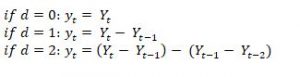
- I: Integrated. The use of differencing of raw observations (e.g. subtracting an observation from an observation at the previous time step) in order to make the time series stationary. ‘d’ is used as a notation to define this component, called the degree of differencing.
- MA: Moving Average. A model that uses the dependency between an observation and a residual error from a moving average model applied to lag observations. ‘q’ is used as a notation to define this component, called the order of moving average.
Identifying the order of differencing in an ARIMA model
The first (and most important) step in fitting an ARIMA model is the determination of the order of differencing needed to make the series stationary. The correct amount of differencing is the lowest order of differencing that yields a time series which fluctuates around a well-defined mean value, standard deviation is lowest and autocorrelation function (ACF) plot decays fairly rapidly to zero, either from above or below.
However, If the series still exhibits a long-term trend, or otherwise lacks a tendency to return to its mean value, or if its autocorrelation are are positive out to a high number of lags (e.g., 10 or more), then this series needs differencing.
An important rule to remember is- If the series has positive autocorrelation out to a high number of lags, then it probably needs a higher order of differencing.
Differencing tends to introduce negative correlation, so if the series initially shows strong positive autocorrelation, then a non-seasonal difference will reduce the autocorrelation and perhaps even drive the lag-1 autocorrelation to a negative value. If you apply a second non-seasonal difference (which is occasionally necessary), the lag-1 autocorrelation will be driven even further in the negative direction.
One of the most common errors in ARIMA modelling is to “over difference” the series and end up adding extra AR or MA terms to undo the damage.
A model with no orders of differencing assumes that the original series is stationary (mean-reverting) know as ARMA model as mentioned earlier.
Identifying the order of AR and MA in an ARIMA model:
After a time series has become stationery by differencing, the next step is to determine whether AR or MA terms are needed to correct any autocorrelation that remains in the differenced series.
By looking at the auto correlation function (ACF) and partial auto correlation (PACF) plots of the differenced series, you can tentatively identify the numbers of AR and/or MA terms that are needed.
ACF plot: it is a bar chart of the coefficients of correlation between a time series and lags of itself.
PACF plot: is a plot of the partial correlation coefficients between the series and lags of itself.
A general ARIMA forecasting equation can be expressed as:
![]()
Understanding basic models for ARIMA:
- ARIMA (1,0,0): first-order Autoregressive model- if the series is stationary and auto correlated, perhaps it can be predicted as a multiple of its own previous value, plus a constant.
![]()
- ARIMA (2,0,0): the series can be said to be dependent on its previous two values.
![]()
- ARIMA (0,1,0): random walk: If the series Y is not stationary, the simplest possible model for it is a random walk model, which can be considered as a limiting case of an AR(1) model in which the autoregressive coefficient is equal to 1, i.e., a series with infinitely slow mean reversion.
![]()
- ARIMA (1,1,0): differenced first-order autoregressive model: If the errors of a random walk model are auto correlated, perhaps the problem can be fixed by adding one lag of the dependent variable to the prediction equation-i.e., by regressing the first difference of Y on itself lagged by one period. This would yield the following prediction equation
![]()
- ARIMA (0,1,1): without constant Moving average model and cab expressed as-
![]()


